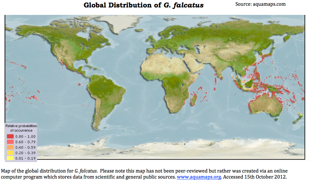
Biogeographic distribution
Natural Distribution of Stomatopods
The natural distribution of G. falcatus stretches from depths of 10m, inter- to subtidal,rocky and coral reef habitats.
The species has been recorded from The Red Sea across the Indo-Pacific Ocean. Countries in which it is most commonly sighted include Australia, Japan throughout the isles of Hawai'i and throughout French Polynesia (Ahyong, 2001). According to molecular data, G. aloha, once thought to be morphologically similar but genetically distinct is now considered conspecific with G. falcatus (Ahyong,2001). One theory explaining the occurance of G.falcatus in Hawai’i is that it was introduced from the Phillipines after World II (Ahyong, 2001).
Anthropogenic introduction of the species throughout theworld is a strong possibility, as the species is a frequent by-catch of the fishing industry. In addition, mantis shrimps are often collected within the live rock sold for the aquarium trade.
Current Research on Stomatopod Biogeography
Larvae ‘not realising its potential’
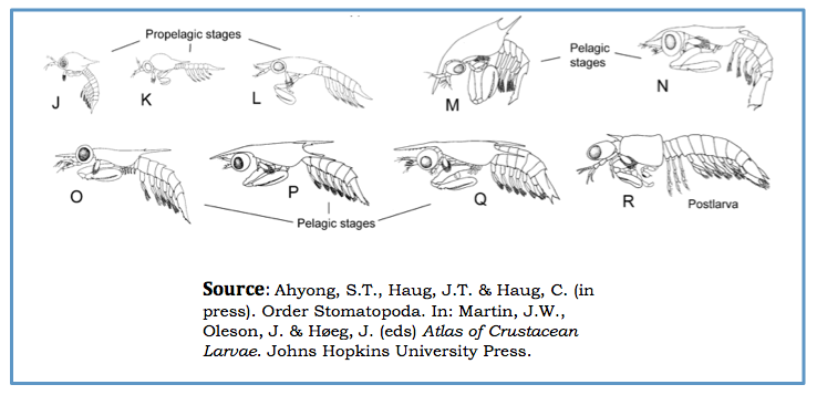
The larval history of an organism has long been thought to play a significant role in the dispersal potential of a species. It was widely held that the longer the larval stage, the further the ‘realisation’ of its dispersal (Shanks et al., 2001). While stomatopods, G. falcatus included, are known to have a planktonic larval phase (Michel, 1970), it has been observed in both fish and invertebrates that suprisingly, larvae migrate only short distances (Burton & Feldman, 1982; Swearer et al., 1999; Jones et al., 1999 in Barber et al, 2002). This, therefore seriously challenges the notion that dispersal potential is fully realised in marine populations (Barber et al., 2000).
Strong ocean currents could well be assumed to spread the larvae of G. falcatus great distances, however one species of stomatopod has displayed surprising genetic differences between seemingly connected ocean currents, indicating a dispersal potential falling far short of its estimated 600km range (Barber et al., 2000). Let's examine some theories as to why this may be the case.

What would be restricting gene flow in the oceans of western and eastern Indonesia?
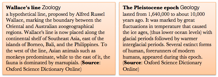
The existence of a marine version of 'Wallace's Line'- the invisible terrestrial delineation between western and eastern Indonesia- has been proposed (Barber et al., 2000). It is suggested that this marine Wallace’s Line may have caused the genetic distinction within a related genus of stomatopod, Haptosquilla in waters seemingly connected by strong ocean currents (Barber et al., 2000).
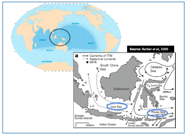
The figure above depicts the direction of key ocean currents with dots representing Marine Protected Areas (MPA), unbroken lines representing the Indonesian Flowthrough (IFT), broken lines depicting seasonal currents. Perpendicular to the terrestrial Wallace’s Line, a genetic break in populations to the north and south of Java and Flores Seas was discovered in stomatpod populations. Northern populations labelled A-G and southern populations are labelled H-K. Source: Barber et al., 2000 Copyright Nature
This biogeographic boundary, this invisible marine ‘Wallace’s Line’ may therefore separate and restrict gene flow.
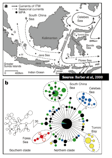
Figure B above represents genetic differences within the 11 regions in Indonesia West Pacific. Mitochrondrial haplotypes (see below) were used in the analysis. Open circles represent northern populations while closed are from south. The relative size of circles is proportional to the frequency of particular haplotypes (or indicated by hash marks or numerals), thus a large closed circle represents a large genetic similarity to another individual in the northern area.
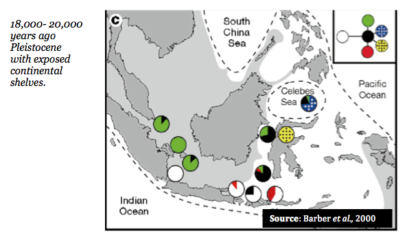
In addition, these genetic distinctions appear to follow the same geographic patterns as experienced during ocean levels during the Pleistocene epoch (~ 1.5 million – 10,000 years ago) when the ocean levels were significantly lower in particular, when the Sunda and Suhul contintental shelves were exposed (18,000- 20,000 years ago).
The figure below depicts the area of this exposed continental shelf shaded grey with the dotted lines indicated the formation of the sea while pie diagrams represent relative frequences of unique mitochondrial haplotypes (again, cytochrome oxidase I).
Dispersal, and consequently species' current distribution and connectivity, should thus be examined in light of both biogeography and broader oceanographic historical time scales (Barber et al., 2000)
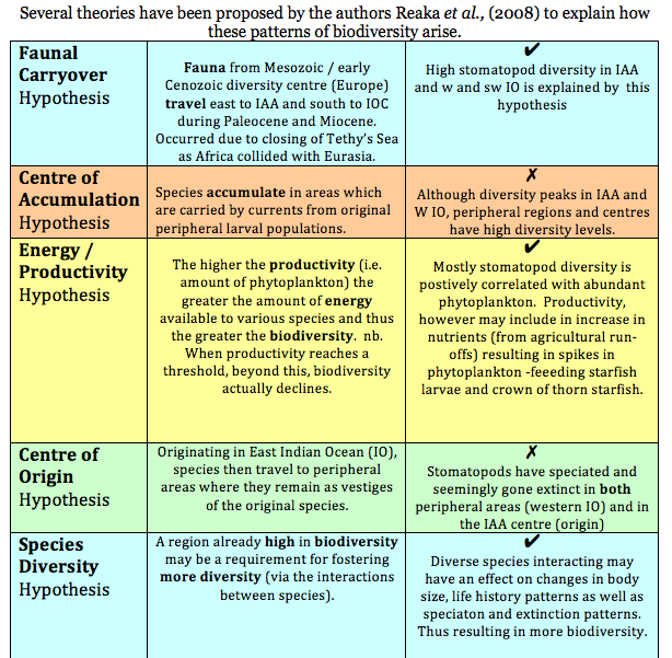
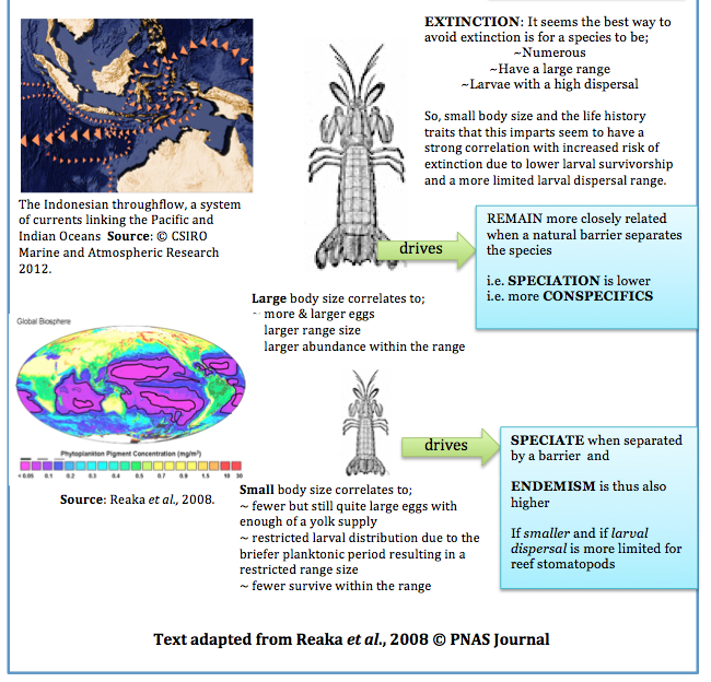
Theories explaining biodiversity (Reaka et al., 2008)
When examining issues of biodiversity on coral reefs really fascinating questions can be raised such as;
What are the patterns of biodiversity on coral reefs?
What factors drive these patterns?
Do high levels of endemism affect biodiversity?
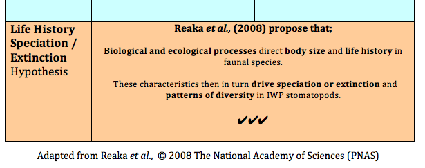
How does life history attributes affect biodiversity? i.e. factors such as body size, range size, abundance, larval stages.
What aspects of the long-term biogeographical history would drive high levels of biodiversity?
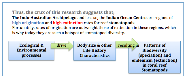
Within the Indonesian West Pacific (IWP) Reaka et al. (2008) draw on what is considered one of the “most ecologically important” taxa of reef animals, the stomatopods, in exploring several theories which may explain patterns of biodiversity.
Several families of stomatopod were collected in the analysis of biodiversity (i.e. Alainosquillidae, Gonodactylidae, Odontodactylidae, Protosquillidae and Takuidae).
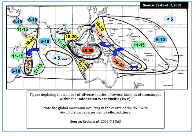
According to research, stomatopod species’ richness appears to follow this pattern;
1. Global maximum in Indo-Australian Archipelago (IAA) with 46-50 species present
2. Biodiversity declines slightly in West Pacific (WP) with 26-30 species present
3. Biodiversity declines yet further in theIndian Ocean (IO) and North-Western IO (Phillipines and Japan) with a second peak at Madagascar and a third peak just south of the IAA, declining with 21-25 species
4. Biodiversity declines further in the Carbibean and Central Pacific (CP) with 11-15 species
|